Analysis of Series of Experiments in Randomized Block Designs
Generally, a single factor experiment is conducted over a number of locations/seasons/years for crop improvement programmes. The objective is to study the performance of treatment effects over different locations/time, aiming to identify treatments suitable for particular environments. The performance of crops generally depends on treatment, environment, and treatment × environment interactions.
Pooled ANOVA
Pooled ANOVA is used to check the existence of treatment × environment interactions. Highly significant interactions indicate that the treatments interacted considerably with environmental changes. In cases where experiments are repeated over time, combined analysis of data is conducted with the following objectives:
- To draw conclusions regarding the suitability of treatments
- To recommend a new variety or fertilizer dose after conducting series of experiments
- To identify technologies whose average effects over years are stable and high
- To reveal the differential response of genotypes to environmental changes
- To study genetic diversity among the genotypes used in an experiment
- To check whether yield trends throughout the experimental period are significantly different from zero
Series of Experiments
Series of experiments are generally conducted in two ways:
- Over seasons/environments
- Over years
Experiments over seasons/environments
For a given crop at a specific site, planting is usually not spread uniformly over a year but bunched to determine whether a separate technology recommendation is needed for each planting season. In such experiments, the objective of pooled analysis over seasons is to examine the interaction between season and treatment.
Experiments over years
The variability of the environment over years is usually unpredictable. Thus, the objective of pooled analysis over years is to identify technologies whose average effect over years is stable and high.
Procedure for Pooled Analysis
The procedure for pooled analysis is as follows:
- Conduct individual analysis for each season, year, or location.
- Compute the error mean square (MSE) values for each season/year/location.
- Test the homogeneity of error variances using Hartley’s test or Bartlett’s chi-square test.
- If error variances are homogeneous, proceed with pooled analysis.
- If error variances are heterogeneous, perform weighted analysis.
Interpretation of Results
1. Homogeneity of Error Variances is Established
a) Check the significance of season, treatment, and interaction. If both treatment and its interaction with season/year are significant, it can be concluded that there is a significant response to treatment, but the response differed between seasons.
b) If season × treatment interaction is significant, partition the interaction sum of squares (SS) into orthogonal contrasts to understand the nature of the interaction.
2. Homogeneity of Error Variances is Not Established
When error variances differ significantly, transform the data by dividing each observation by the square root of the MSE of the environment before performing the combined analysis.
Output of the Program
The output of this module includes:
- Means of treatments for different seasons/years in tabular form
- Separate ANOVA for each season/year
- Bartlett’s test statistics with significance
- Combined ANOVA for pooled data
- Broad interpretation of results
Procedure for Data Entry
A data entry page is provided where users can input data as well as year/season names. Data for all replications of the first treatment for the first year/season must be entered in the first row, with each value separated by at least one space. After entering data for the first treatment, enter data for subsequent treatments and seasons in a similar manner. Data can be copied from Excel and pasted into the interface.
Example: The dataset for a varietal trial conducted to study the performance of nine new mustard strains versus three checks, using an RCB design with three replications at each environment, is provided. The seed yield in kg/ha recorded have been taken from the table 8.2 of the book “Statistical Analysis of Agricultural Experiments Part I: Single Factor Experiments” by Gupta et al. 2016) ICAR-IASRI, Library Avenue, Pusa, New Delhi.
Data of Grain yield of rice tested with five rates of nitrogen over two seasons.
____________________________________________________________________________________________

Environ		Treat	     Replication	Environ		Treat	    Replication
                        ___________________				____________________
			1	2	3				1	2	3
____________________________________________________________________________________________
Bathinda	1	1794	2014	2581	Hisar		1	3286	2459	3286
		2	1134	1736	1898			2	2518	2364	2364
		3	718	764	880			3	757	993	875
		4	1852	1551	1887			4	2553	2388	2884
		5	2245	2361	2407			5	2908	2482	2884
		6	1111	1065	1111			6	1797	1560	2033
		7	1181	880	1528			7	1749	1537	1537
		8	1644	1991	2060			8	1501	2317	2577
		9	1551	1435	1991			9	1513	1608	2104
		10	1968	1551	2569			10	2447	2459	2813
		11	2662	2338	3056			11	2600	2884	2648
		12	1065	1227	1343			12	1631	1466	1844

IARI New Delhi	1	2600	2444	2711	Ludhiana	1	1370	1209	1320
		2	3289	2667	2889			2	904	729	1007
		3	2756	2511	2400			3	858	942	839
		4	2600	2444	2222			4	904	959	1155
		5	2689	2422	2444			5	1438	1456	1695
		6	2578	2400	2222			6	873	959	946
		7	3178	3044	2889			7	848	639	643
		8	3244	2911	3111			8	1668	1770	1607
		9	2444	2222	2667			9	910	907	1081
		10	3156	2978	2756			10	1558	1606	1705
		11	2667	2267	2111			11	1508	1389	1447
		12	2689	2444	2289			12	1280	1207	1256

Navgaon		1	2233	2222	2222	TERI,New Delhi	1	1666	1333	2222
		2	2222	2444	2722			2	1611	1389	1944
		3	2000	1778	1778			3	1389	1244	2056
		4	2667	3289	3333			4	1511	1778	1889
		5	2444	2000	2000			5	1644	1622	1711
		6	1778	1889	1556			6	1833	1822	2111
		7	1778	1722	1722			7	1788	2333	1711
		8	3000	2889	3222			8	1644	2220	2220
		9	1778	1611	1333			9	1889	1822	2444
		10	3778	3667	3556			10	2000	1556	1356
		11	3111	3111	3222			11	944	388	722
		12	2222	2000	2222			12	1488	1400	1356
_______________________________________________________________________________________________
Using the above Example you have arrange the data in text area as give under :
1794	2014	2581
1134	1736	1898
718	764	880
1852	1551	1887
2245	2361	2407
1111	1065	1111
1181	880	1528
1644	1991	2060
1551	1435	1991
1968	1551	2569
2662	2338	3056
1065	1227	1343
2600	2444	2711
3289	2667	2889
2756	2511	2400
2600	2444	2222
2689	2422	2444
2578	2400	2222
3178	3044	2889
3244	2911	3111
2444	2222	2667
3156	2978	2756
2667	2267	2111
2689	2444	2289
2233	2222	2222
2222	2444	2722
2000	1778	1778
2667	3289	3333
2444	2000	2000
1778	1889	1556
1778	1722	1722
3000	2889	3222
1778	1611	1333
3778	3667	3556
3111	3111	3222
2222	2000	2222
3286	2459	3286
2518	2364	2364
757	993	875
2553	2388	2884
2908	2482	2884
1797	1560	2033
1749	1537	1537
1501	2317	2577
1513	1608	2104
2447	2459	2813
2600	2884	2648
1631	1466	1844
1370	1209	1320
904	729	1007
858	942	839
904	959	1155
1438	1456	1695
873	959	946
848	639	643
1668	1770	1607
910	907	1081
1558	1606	1705
1508	1389	1447
1280	1207	1256
1666	1333	2222
1611	1389	1944
1389	1244	2056
1511	1778	1889
1644	1622	1711
1833	1822	2111
1788	2333	1711
1644	2220	2220
1889	1822	2444
2000	1556	1356
944	388	722
1488	1400	1356
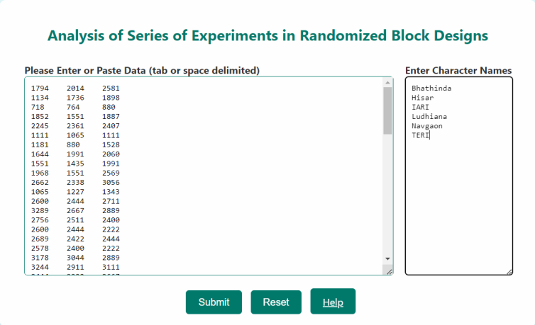
Step 1:The entered data in the data entry web page looks as under:-

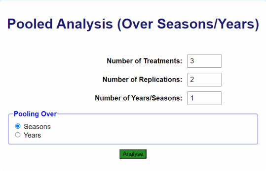
Step 1:After entering the data and locations/years/seasons name press “Submit” button. Another web page will be displayed as given below:-

Step 2: Enter the number of treatments, number of replications and number of years/seasons in the text boxes provided. Also select seasons or year from the option buttons as per your requirements. After filling all the required information press “Analyse” button. The results will be displayed on separate web page.